Introducing Logistic Falkon

Introduction

In this notebook we use a synthetic dataset to show how the LogisticFalkon estimator works.

We compare Falkon – which is trained on the squared loss – to its logistic loss version, and verify that on a binary classification problem logistic falkon achieves better accuracy.

%matplotlib inline
from sklearn import datasets, model_selection
import torch
import matplotlib.pyplot as plt
plt.style.use('ggplot')

import falkon

[pyKeOps]: Warning, no cuda detected. Switching to cpu only.

Load the data

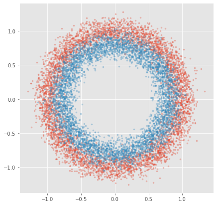
We use a synthetic dataset in two dimensions, which consists of two concentric circles labeled with different classes.

We introduce quite a bit of noise so that the estimators will not trivially achieve zero error, and we draw 10000 samples to demonstrate the speed of the Falkon library.

X, Y = datasets.make_circles(
    n_samples=10_000, shuffle=False, noise=0.1, random_state=122)

fig, ax = plt.subplots(figsize=(7, 7))
ax.scatter(X[Y == 0,0], X[Y == 0,1], alpha=0.3, marker='.')
_ = ax.scatter(X[Y == 1,0], X[Y == 1,1], alpha=0.3, marker='.')

Split into training and test sets

We split the data into a training set with 80% of the samples and a test set with the remaining 20%.

X_train, X_test, Y_train, Y_test = model_selection.train_test_split(
    X, Y, test_size=0.2, random_state=10, shuffle=True)

Data Preprocessing

The minimal preprocessing steps are: 1. Convert from numpy arrays to torch tensors 2. Convert data and labels to the same data-type (in this case float32) 3. Reshape the labels so that they have two dimensions. This is not strictly necessary, but Falkon internally works with 2D tensors, so the output of the Falkon.predict method will always be 2D. 4. Change the labels from 0, 1 to -1, 1. Note that Logistic Falkon uses the following formula for the logistic loss:

\[\log(1 + e^{-y_1 y_2})\]

where $y_1$ and $y_2$ are labels and predictions respectively, which only makes sense if the labels are -1, 1.

X_train = torch.from_numpy(X_train).to(dtype=torch.float32)
X_test = torch.from_numpy(X_test).to(dtype=torch.float32)
Y_train = torch.from_numpy(Y_train).to(dtype=torch.float32).reshape(-1, 1)
Y_test = torch.from_numpy(Y_test).to(dtype=torch.float32).reshape(-1, 1)

Y_train[Y_train == 0] = -1
Y_test[Y_test == 0] = -1

Define the Falkon model

We use the same base parameters for both models: a small amount of regularization (\(10^{-7}\)) and a Gaussian kernel with \(\sigma = 5\). The number of inducing points is set to 1000 which is adequate for the problem which is very easy.

def binary_loss(true, pred):
    return torch.mean((true != torch.sign(pred)).to(torch.float32))

# We define some basic options to run on the CPU, and to disable keops
flk_opt = falkon.FalkonOptions(use_cpu=True, keops_active="no")

flk_kernel = falkon.kernels.GaussianKernel(1, opt=flk_opt)

flk = falkon.Falkon(kernel=flk_kernel, penalty=1e-7, M=1000, options=flk_opt)

Define Logistic Falkon model

The logistic Falkon estimator uses the same base parameters as Falkon.

However, instead of specifying a single value for regularization, we need to specify a regularization path: a series of decreasing amounts of regularization. For each regularization value we also need to specify the number of iterations of conjugate gradient descent, which will be performed for that specific regularization value.

We validated empirically on a wide number of binary classification problems that a good scheme to set the regularization path is to use three short (i.e. 3 iterations) runs with increasing regularization, and then a few longer (here we used 8 iterations) runs with the final regularization value (here 1e-7, the same as for Falkon).

The LogisticFalkon estimator also accepts a mandatory loss parameter, which should be set to an instance of the LogisticLoss class. While the LogisticLoss is the only implemented loss at the moment, the learning algorithm is defined for any generalized self-concordant loss, and we plan to extend the library to support more functions.

An additional feature we show here is error monitoring: By passing an error function to the estimator (see parameter error_fn), the estimator will print the training error at every iteration (how often such prints occur is governed by the error_every parameter). This can be very useful to determine if it is possible to stop training early, and in general to monitor the training process.

logflk_opt = falkon.FalkonOptions(use_cpu=True, keops_active="no")

logflk_kernel = falkon.kernels.GaussianKernel(1, opt=logflk_opt)
logloss = falkon.gsc_losses.LogisticLoss(logflk_kernel)

penalty_list = [1e-3, 1e-5, 1e-7, 1e-7, 1e-7]
iter_list = [4, 4, 4, 8, 8]

logflk = falkon.LogisticFalkon(
    kernel=logflk_kernel, penalty_list=penalty_list, iter_list=iter_list, M=1000, loss=logloss,
    error_fn=binary_loss, error_every=1, options=logflk_opt)

Train both models

Training Falkon for 20 iterations (default value) takes about half a secon on a laptop.

Clearly, since the logistic falkon runs about 28 iterations (the sum of values in iter_list), it is necessarily going to be slower. Further, logistic falkon needs to recompute part of the preconditioner at every step of the Newton method leading to further slowdowns. On the same laptop, the logistic falkon algorithm takes around 1.5s.

%%time
flk.fit(X_train, Y_train);

CPU times: user 2.35 s, sys: 59.3 ms, total: 2.41 s
Wall time: 604 ms

Falkon(M=1000, center_selection=<falkon.center_selection.UniformSelector object at 0x7f9f7d142b20>, kernel=GaussianKernel(sigma=Parameter containing:
tensor([1.], dtype=torch.float64)), options=FalkonOptions(keops_acc_dtype='auto', keops_sum_scheme='auto', keops_active='no', keops_memory_slack=0.7, chol_force_in_core=False, chol_force_ooc=False, chol_par_blk_multiplier=2, pc_epsilon_32=1e-05, pc_epsilon_64=1e-13, cpu_preconditioner=False, cg_epsilon_32=1e-07, cg_epsilon_64=1e-15, cg_tolerance=1e-07, cg_full_gradient_every=10, cg_differential_convergence=False, debug=False, use_cpu=True, max_gpu_mem=inf, max_cpu_mem=inf, compute_arch_speed=False, no_single_kernel=True, min_cuda_pc_size_32=10000, min_cuda_pc_size_64=30000, min_cuda_iter_size_32=300000000, min_cuda_iter_size_64=900000000, never_store_kernel=False, store_kernel_d_threshold=1200, num_fmm_streams=2), penalty=1e-07)

%%time
logflk.fit(X_train, Y_train);

Iteration 0 - penalty 1.000000e-03 - sub-iterations 4
Iteration   0 - Elapsed 0.27s - training loss 0.4697 - training error 0.1544
Iteration 1 - penalty 1.000000e-05 - sub-iterations 4
Iteration   1 - Elapsed 0.51s - training loss 0.3774 - training error 0.1551
Iteration 2 - penalty 1.000000e-07 - sub-iterations 4
Iteration   2 - Elapsed 0.74s - training loss 0.3575 - training error 0.1534
Iteration 3 - penalty 1.000000e-07 - sub-iterations 8
Iteration   3 - Elapsed 1.12s - training loss 0.3554 - training error 0.1530
Iteration 4 - penalty 1.000000e-07 - sub-iterations 8
Iteration   4 - Elapsed 1.50s - training loss 0.3554 - training error 0.1530
CPU times: user 6.39 s, sys: 30.9 ms, total: 6.42 s
Wall time: 1.6 s

LogisticFalkon(M=1000, center_selection=<falkon.center_selection.UniformSelector object at 0x7f9f7d150250>, error_fn=<function binary_loss at 0x7f9f7d13eaf0>, iter_list=[4, 4, 4, 8, 8], kernel=GaussianKernel(sigma=Parameter containing:
tensor([1.], dtype=torch.float64)), loss=LogisticLoss(kernel=GaussianKernel(sigma=Parameter containing:
tensor([1.], dtype=torch.float64))), options=FalkonOptions(keops_acc_dtype='auto', keops_sum_scheme='auto', keops_active='no', keops_memory_slack=0.7, chol_force_in_core=False, chol_force_ooc=False, chol_par_blk_multiplier=2, pc_epsilon_32=1e-05, pc_epsilon_64=1e-13, cpu_preconditioner=False, cg_epsilon_32=1e-07, cg_epsilon_64=1e-15, cg_tolerance=1e-07, cg_full_gradient_every=10, cg_differential_convergence=False, debug=False, use_cpu=True, max_gpu_mem=inf, max_cpu_mem=inf, compute_arch_speed=False, no_single_kernel=True, min_cuda_pc_size_32=10000, min_cuda_pc_size_64=30000, min_cuda_iter_size_32=300000000, min_cuda_iter_size_64=900000000, never_store_kernel=False, store_kernel_d_threshold=1200, num_fmm_streams=2), penalty_list=[0.001, 1e-05, 1e-07, 1e-07, 1e-07])

Testing

However, the price paid for with a higher training time, leads to lower training error.

We found that, on a variety of binary classification datasets, logistic falkon obtains a slightly lower error than the vanilla Falkon algorithm.

flk_pred = flk.predict(X_test)
flk_err = binary_loss(Y_test, flk_pred)

logflk_pred = logflk.predict(X_test)
logflk_err = binary_loss(Y_test, logflk_pred)

print("Falkon model          -- Error: %.2f%%" % (flk_err * 100))
print("Logistic Falkon model -- Error: %.2f%%" % (logflk_err * 100))

Falkon model          -- Error: 17.05%
Logistic Falkon model -- Error: 16.90%

Plot predictions

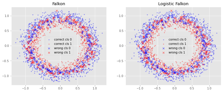
In the plot we have the outer and inner circles which are correct predictions, and the circles in the middle which are the mispredicted points. Since we added lots of noise to the dataset, perfect predictions are not possible (there is no clear boundary between the two classes).

Here the error difference between Falkon and Logistic Falkon is very hard to distinguish by eye. However, there may be other applications where the best possible classification error is desired.

def plot_predictions(preds, ax):
    ax.scatter(X_test[((Y_test == -1) & (preds.sign() == Y_test)).reshape(-1), 0],
               X_test[((Y_test == -1) & (preds.sign() == Y_test)).reshape(-1), 1],
               alpha=0.3, marker='.', color='b', label="correct cls 0")
    ax.scatter(X_test[((Y_test == 1) & (preds.sign() == Y_test)).reshape(-1),0],
               X_test[((Y_test == 1) & (preds.sign() == Y_test)).reshape(-1),1],
               alpha=0.3, marker='.', color='r', label="correct cls 1")

    ax.scatter(X_test[((Y_test == -1) & (preds.sign() != Y_test)).reshape(-1), 0],
               X_test[((Y_test == -1) & (preds.sign() != Y_test)).reshape(-1), 1],
               alpha=0.5, marker='x', color='b', label="wrong cls 0")
    ax.scatter(X_test[((Y_test == 1) & (preds.sign() != Y_test)).reshape(-1),0],
               X_test[((Y_test == 1) & (preds.sign() != Y_test)).reshape(-1),1],
               alpha=0.5, marker='x', color='r', label="wrong cls 1")

fig, ax = plt.subplots(ncols=2, figsize=(13, 5))
plot_predictions(flk_pred, ax[0])
ax[0].set_title("Falkon")
ax[0].legend(loc='best')

plot_predictions(logflk_pred, ax[1])
ax[1].set_title("Logistic Falkon")
ax[1].legend(loc='best');